In this blog entry, I summarise the recent publication [1], which provides a fully reproducible standard problem. The associated code [2] allows to re-compute and reproduce key figures in the paper by carrying out the required installation, simulation, post-processing and plot creation on the Travis CI service.

[1] Alexander Baker, Marijan Beg, Gregory Ashton, Maximilian Albert, Dmitri Chernyshenko, Weiwei Wang, Shilei Zhang, Marc-Antonio Bisotti, Matteo Franchin, Chun Lian Hu, Robert Stamps, Thorsten Hesjedal, Hans Fangohr Proposal of a micromagnetic standard problem for ferromagnetic resonance simulations Journal of Magnetism and Magnetic Materials 421, 428-439 (2017), arXiv:1603.05419

[2] Electronic supplementary material on Github, DOI:10.5281/zenodo.59714, with full reproducible run at Circle CI

Below, I review the challenge of reproducibility in computational science, and the role of 'standard problems' to help with validation of simulation codes for correctness. I then summarise the above publication in this context, including (i) description of the re-computation process that has been set up on Circle CI, and (ii) a summary of the standard problem validation steps that has been taken in the study.

Introduction reproducible computational science¶

Reproducibility is a key objective in research: results are considered true if they can be reproduced by a different group of researchers, following the description of the work of the first group (for example the description given in a scientific publication).

Currently, there are very few publications in computational science that (can) achieve this gold standard of reproducibly computational science: to achieve reproducibility of computational science studies one needs availability of the simulation codes and the precise version that has been used, the exact configuration for each run, the precise way of post-processing, analysing and plotting data. Furthermore, the results may depend on the operating system, hardware, support libraries and - when parallel execution is involved - the non-deterministic execution order of threads and processes.

Introduction standard problems in micromagnetics¶

In 1995 a number of researchers in the area of magnetic nanostructures (using a technique called computational micromagnetics) got together to develop a strategy to improve correctness in computational micromagnetics (see notes from meetings in April 1995 and November 1995).

A number of simulation problems were proposed and described in such detail that anybody could attempt to carry out that particular simulation, and then compare their own results with those published on in a public repository on the Internet. Each study is known as a standard problem. In other domains comparable efforts are sometimes called benchmarks although (at least in my view) it is the correctness of the simulation results that is more important than the performance (and benchmark is sometimes associated with performance).

Over time, the number of standard problems has grown, the first 5 standard problems are available; a sixth standard problem focussing on magnonics has been propsed in 2012.

This paper¶

In this paper [1], we propose a new standard problem (number 7 if we carry on counting), carry out the calculation and present the results. We also provide configuration files for two open source packages (called OOMMF and Nmag) to carry out the calculation, and all required post-processing scripts to regenerate the results of this standard problem, and key figures in the paper [2].

Making these scripts available is combined with a continuous integration setup (here using Circle CI), where we re-compute the key results (using OOMMF) when the source repository changes, or on demand. Other parties can clone this repository (activate testing via Circle CI for their account), and re-execute the whole computational workflow to produce the key figures and data show in the figure.

The provision of a continuous integration setup goes beyond provision of the required configuration files and post-processing scripts: we provide at least one well defined computing environment in which the simulations and scripts execute. Setting up this environment includes picking a linux distribution, installing of required support libraries, picking a TcL environment and C++ compiler, etc.

What testing and recomputation is done on Circle CI?¶

Before the testing starts, a computational environment is created, in which the OOMMF software and helper libraries are installed. The figure below shows an overview of the testing steps:

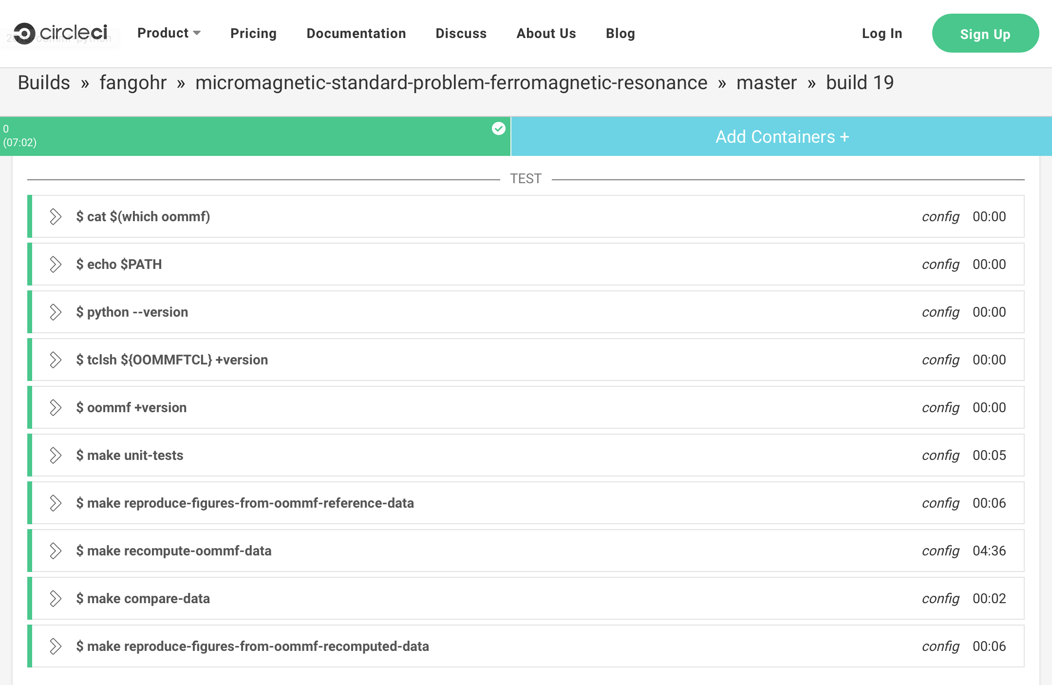
Figure showing an overview of the testing steps carried out of the continuous integration process

The first 5 tasks (cat $(which oommf) to oommf +version) are purely providing additional information on which versions of OOMMF, TcL and Python are being used.

• make unittests runs unit tests for the post-processing code.

• make reproduce-figures-from-oommf-reference-data is a script that will re-create the key figures of the paper, based on data that has in the past computed using OOMMF and is deposited in the repository to be easily availble, if researchers want to validate their own codes against this stored solution of the standard problem.

• make recompute-oommf-data re-computes this data set from scratch (in a different folder).

• make compare-data compares the two data sets (the reference data stored in the repository, and the one that has been recomputed in the previous step) and raises an alerm if the two data sets do not agree.

The last target reproduces the figurse from the recomputed data - this is expected to give the same figure as those create from the reference data, as the previous step ensures the two data sets are identical.

For each of the steps, the detailed output can be inspected on the Circle CI testing system webpage.

Details of re-computation environment¶

For the current testing with Circle CI, we use an anaconda environment to set up OOMMF. It would be desirable to also provide an installation and run through the same scripts which is based on manual installation of the OOMMF software on a linux system. This should now be feasible, as the Jupyter-OOMMF project has configuration files that compile OOMMF on Travis CI from the OOMMF source that is hosted at https://github.com/fangohr/oommf. Or to run the same calculation within a Docker container. Pull requests welcome! ;)

What kind of validation is done in the paper?¶

Comparing with analytical result for simplified problem¶

A common approach for simulation validation and testing is to simplify the simulated problem to one where an exact solution can be computed using analytical methods, and to then compare the analytical solution with the numerical one. If there is agreement of the solutions, there is hope that the simulation may be correct. If there is disagreement, there is clearly something wrong.

In this case of ferromagnetic resonance, there is a special case for which the answer is known exactly: that of a magnetic dipole precessing in an applied magnetic field. The micromagnetic problem simplifies to this situation if (i) the magnetisation is pointing in the same direction everywhere initially, and (ii) the demagnetisation effects are ignored. We do then expect that the whole magnetisation remains spatially uniform over time, and precesses with a frequency that can be computed from the applied field. This is demonstrated in Appendix C and equation (B.11) of the paper.

Using two simulation packages¶

To carry out the full simulation, we use two open source packages (OOMMF and Nmag). They have been developed by different teams (that is good for testing), and they use different numerical methods (finite difference versus finite elements for spatial discretisation, different ways of computing the demagnetisation field, and different time integrator schemes).

This 'independence' of the code is generally useful as it avoids making the same mistake in both tools. However, there are also different numerical errors associated with the different methods. In particular in the study here, we have chosen a geometry for which we expect the finite difference code to be very well suited to simulate it (as the method is more widely used). Because of these different approaches, we do find deviation of results between the finite element method and the finite difference based approaches. We have shown that as the mesh is refined in the finite element method, the results approach those of the finite difference method; supporting our hypothesis that both method produce the same results, and that the finite difference method is better suite for this problem (Figure 14).

We restrict the re-computation effort to using the finite difference tool, as it produced the better results in shorter runtime, and is more widely used, and has been used to compute the data for most of the figures in the paper. (We describe in the next section that a completely different computational method produces results that agree very well with the finite difference solution, further supporting our hypothesis.)

Using two different computational methods¶

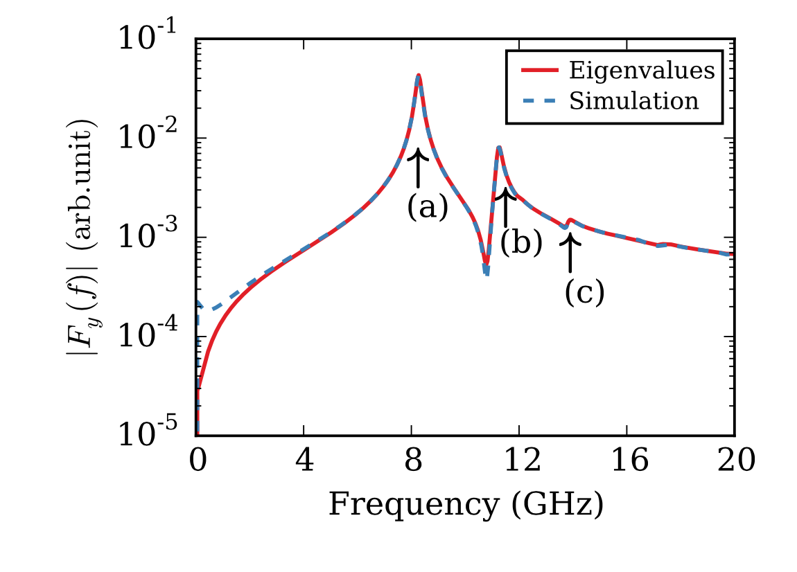
Figure showing ferromagnetic resonance data that has been computed with two completely different methods: the Simulation method (dashed blue line) is exciting with a particular field pulse, and then the time development of the system is simulated for many time steps. Subsequently, fourier transforms of the recorded data are computed which, averaged in the right way, obtain the curve in the figure. The Eigenvalue method is quite different in that the spectrum of frequencies and eigenmodes that the system can show is computed directly through solution of an eigen value problem. It is then computed what kind of frequency response we would expect for the excitation (and the damping value) that is used in the simulation approach. This results in the solid red line.

The deviation beween the two lines in the figure above at low frequencies is expected (as a finite run time for the simulation method will give the more inaccurate results the closer we move to frequency 0). The agreement of the two lines for higher frequencies instills confidence in the correctness of both methods, and thus the results. Unless we have made a mistake in the basic equations to be used, it is very unlikely that this good agreement is achieved by coincidence.