15. Visualising Data#
The purpose of scientific computation is insight not numbers: To understand the meaning of the (many) numbers we compute, we often need postprocessing, statistical analysis and graphical visualisation of our data. The following sections describe
Matplotlib/Pylab — a tool to generate high quality graphs of the type y = f(x) (and a bit more)
the
pylabinterfacethe
pyplotinterface
We also touch on:
Visual Python — a tool to quickly generate animations of time dependent processes taking place in 3d space.
Tools to store and visualise vtk files
We close with a short outlook on
Further tools and developments discussing other tools and emerging approaches for data visualisation and analysis.
15.1. Matplotlib – plotting y=f(x), (and a bit more)#
The Python library Matplotlib is a python 2D plotting library which produces publication quality figures in a variety of hardcopy formats and interactive environments. Matplotlib tries to make easy things easy and hard things possible. You can generate plots, histograms, power spectra, bar charts, errorcharts, scatterplots, etc, with just a few lines of code.
For more detailed information, check these links
A very nice introduction in the object oriented Matplotlib interface, and summary of all important ways of changing style, figure size, linewidth, etc. This is a useful reference: jrjohansson/scientific-python-lectures
Extended thumbnail gallery of examples https://matplotlib.org/stable/gallery/index.html
15.1.1. Matplotlib and Pylab#
The Matplotlib package provides an object oriented plotting library under the name space matplotlib.pyplot.
The pylab interface is provided through the Matplotlib package. Internally it uses matplotlib.pyplot functionality but imitates the (state-driven) Matlab plotting interface.
The pylab interface is slightly more convenient to use for simple plots, and matplotlib.pyplot gives far more detailed control over how plots are created. If you routinely need to produce figures, we suggest to learn about the object oriented matplotlib.pyplot interface (instead of the pylab interface).
This chapter focusses on the Pylab interface, but also provides examples for the object-oriented matplotlib.pyplot interface.
An excellent introduction and overview of the matplotlib.pyplot plotting interface is available in jrjohansson/scientific-python-lectures.
For the purpose of this book and the Jupyterbook package, we use some settings to create a svg file for the html version of the book, and a high-resolution png file for the pdf version:
%matplotlib inline
# settings for jupyter book: svg for html version, high-resolution png for pdf
import matplotlib_inline
matplotlib_inline.backend_inline.set_matplotlib_formats('svg', 'png')
import matplotlib as mpl
mpl.rcParams['figure.dpi'] = 400
15.1.2. First example#
15.1.2.1. The pyplot interface#
The recommended way of using Matplotlib in a simple example is shown here:
# example 1 a
import numpy as np                  # get access to fast arrays
import matplotlib.pyplot as plt     # the plotting functions

x = np.arange(-3.14, 3.14, 0.01)    # create x-data
y = np.sin(x)                       # compute y-data
plt.plot(x, y)                      # create plot
[<matplotlib.lines.Line2D at 0x7fc840326890>]

15.1.3. How to import matplotlib, pylab, pyplot, numpy and all that#
The submodule matplotlib.pyplot provides an object oriented interface to the plotting library. Many of the examples in the matplotlib documentation follow the import convention to import matplotlib.pyplot as plt and numpy as np. It is of the user’s decision whether to import the numpy library under the name np (as often done in matplotlib examples) or N as occasionally done in this text (and in the early days when the predecessor of numpy was called “Numeric”) or any other name you like. Similarly, it is a matter of taste whether the plotting submodule (matplotlib.pyplot) is imported as plt as is done in the matplotlib documentation or plot (which could be argued is slightly clearer) etc.
As always a balance has to be struck between personal preferences and consistency with common practice in choosing these name. Consistency with common use is more important if the code is likely to be used by others or published.
15.1.3.1. The Pylab interface#
We introduce the pylab interface by translating the example 1a above to the following example 1b (which is identical in functionality to the example 1a and will create the same plot):
# example 1b
import pylab
import numpy as np

x = np.arange (-3.14, 3.14, 0.01)
y = np.sin(x)

pylab.plot(x, y)
[<matplotlib.lines.Line2D at 0x7fc84029b550>]

Plotting nearly always needs arrays of numerical data and it is for this reason that the numpy module is used a lot: it provides fast and memory efficient array handling for Python (see chapter 14). The pylab interface has taken this a step further and automatically imports all objects from numpy into the pylab name space:
Because the numpy.arange and numpy.sin objects have already been imported into the pylab namespace, we could also write it as example 1c:
# example 1c
import pylab as p

x = p.arange(-3.14, 3.14, 0.01)
y = p.sin(x)

p.plot(x, y)
[<matplotlib.lines.Line2D at 0x7fc84011b950>]

If we really want to cut down on characters to type, we could also important all the objects (*) from the pylab convenience module into our current namespace, and rewrite the code as example 1d:
# example 1 d
from pylab import *  # not generally recommended
                     # okay for interactive testing

x = arange(-3.14, 3.14, 0.01)
y = sin(x)
plot(x, y)
show()

This can be extremely convenient, but comes with a big health warning:
While using
from pylab import *is acceptable at the command prompt to interactively create plots and analyse data, this should never be used in any plotting scripts.The pylab toplevel provides over 800 different objects which are all imported into the global name space when running
from pylab import *. This is not good practice, and could conflict with other objects that exist already or are created later.As a rule of thumb: do never use
from somewhere import *in programs we save. This may be okay at the command prompt for interactive data exploration.
15.1.4. IPython’s inline mode#
Within the Jupyter Notebook or Qtconsole (see the Python shells notebook) we can use the %matplotlib inline magic command to make further plots appear within our console or notebook. To force pop up windows instead, use %matplotlib qt.
If you enjoy the pylab interface, then you maybe interested in the %pylab magic, which will not only switch to inline plotting but also automatically execute from pylab import *.
15.1.5. Saving the figure to a file#
Once you have created the figure (using the plot command) and added any labels, legends etc, you have two options to save the plot.
You can display the figure (using
show) and interactively save it by clicking on the disk icon. (This does not work with inline plots as the icons are not available.)You can (without displaying the figure) save it directly from your Python code. The command to use is
savefig. The format is determined by the extension of the file name you provide. Here is an example (pylabsavefig.py) which saves a figure into different files.
# saving figure files with the pylab interface
import pylab
import numpy as np

x = np.arange(-3.14, 3.14, 0.01)
y = np.sin(x)

pylab.plot(x, y, label='sin(x)')
pylab.savefig('myplot.png')  # saves png file
pylab.savefig('myplot.svg')  # saves svg file
pylab.savefig('myplot.eps')  # saves svg file
pylab.savefig('myplot.pdf')  # saves pdf file
pylab.close()
A note on file formats:
The pdf, eps and svg file formats are vector file formats which means that one can zoom into the image without loosing quality (lines will still be sharp). File formats such as png (and jpg, gif, tif, bmp) save the image in form of a bitmap (i.e. a matrix of colour values) and will appear blurry or pixelated when zooming in (or when printed in high resolution).
Accordingly, choose a vector file format where you can, and use the bitmap (png for example) if there are no other options. Choose the eps or pdf file format if you plan to include the figure in a Latex document – depending on whether you want to compile it using latex (needs eps) or pdflatex (can use pdf [better] or png). If the version of MS Word (or other text processing software you use) can handle pdf files, it is better to use pdf than png for that.
# saving figure files with the pyplot interface
from matplotlib import pyplot as plt
import numpy as np

x = np.arange(-3.14, 3.14, 0.01)
y = np.sin(x)

fig, ax = plt.subplots()
ax.plot(x, y, label='sin(x)')
fig.savefig('myplot.png')  # saves png file
fig.savefig('myplot.svg')  # saves svg file
fig.savefig('myplot.eps')  # saves svg file
fig.savefig('myplot.pdf')  # saves pdf file
plt.close(fig)
15.2. The pylab interface#
15.2.1. Fine tuning your plot#
Matplotlib allows us to fine tune our plots in great detail. Here is an example:
import pylab
import numpy as N

x = N.arange(-3.14, 3.14, 0.01)
y1 = N.sin(x)
y2 = N.cos(x)
pylab.figure(figsize =(5 , 5))
pylab.plot(x, y1, label='sin(x)')
pylab.plot(x, y2, label='cos(x)')
pylab.legend()
pylab.axis([-2, 2, -1, 1])
pylab.grid()
pylab.xlabel('x')
pylab.title('This is the title of the graph')
Text(0.5, 1.0, 'This is the title of the graph')

showing some other useful commands:
figure(figsize=(5, 5))sets the figure size to 5inch by 5inchplot(x, y1, label=’sin(x)’)The “label” keyword defines the name of this line. The line label will be shown in the legend if thelegend()command is used later.Note that calling the
plotcommand repeatedly, allows you to overlay a number of curves.axis([-2, 2, -1, 1])This fixes the displayed area to go from xmin=-2 to xmax=2 in x-direction, and from ymin=-1 to ymax=1 in y-directionlegend()This command will display a legend with the labels as defined in the plot command. Tryhelp(pylab.legend)to learn more about the placement of the legend.grid()This command will display a grid on the backdrop.xlabel(’...’)andylabel(’...’)allow labelling the axes.
Note further than you can chose different line styles, line thicknesses, symbols and colours for the data to be plotted. (The syntax is very similar to MATLAB.) For example:
plot(x, y, ’og’)will plot circles (o) in green (g)plot(x, y, ’-r’)will plot a line (-) in red (r)plot(x, y, ’-b’, linewidth=2)will plot a blue line (b) with two two pixel thicknesslinewidth=2which is twice as wide as the default.plot(x, y, ’-’, alpha=0.5)will plot a semi-transparent line (b).
The full list of options can be found when typing help(pylab.plot) at the Python prompt. Because this documentation is so useful, we repeat parts of it here:
plot(*args, **kwargs)
    Plot lines and/or markers to the
    :class:`~matplotlib.axes.Axes`.  *args* is a variable length
    argument, allowing for multiple *x*, *y* pairs with an
    optional format string.  For example, each of the following is
    legal::

        plot(x, y)         # plot x and y using default line style and color
        plot(x, y, 'bo')   # plot x and y using blue circle markers
        plot(y)            # plot y using x as index array 0..N-1
        plot(y, 'r+')      # ditto, but with red plusses

    If *x* and/or *y* is 2-dimensional, then the corresponding columns
    will be plotted.

    An arbitrary number of *x*, *y*, *fmt* groups can be
    specified, as in::

        a.plot(x1, y1, 'g^', x2, y2, 'g-')

    Return value is a list of lines that were added.

    The following format string characters are accepted to control
    the line style or marker:

    ================    ===============================
    character           description
    ================    ===============================
    '-'                 solid line style
    '--'                dashed line style
    '-.'                dash-dot line style
    ':'                 dotted line style
    '.'                 point marker
    ','                 pixel marker
    'o'                 circle marker
    'v'                 triangle_down marker
    '^'                 triangle_up marker
    '<'                 triangle_left marker
    '>'                 triangle_right marker
    '1'                 tri_down marker
    '2'                 tri_up marker
    '3'                 tri_left marker
    '4'                 tri_right marker
    's'                 square marker
    'p'                 pentagon marker
    '*'                 star marker
    'h'                 hexagon1 marker
    'H'                 hexagon2 marker
    '+'                 plus marker
    'x'                 x marker
    'D'                 diamond marker
    'd'                 thin_diamond marker
    '|'                 vline marker
    '_'                 hline marker
    ================    ===============================

The following color abbreviations are supported:

==========  ========
character   color
==========  ========
'b'         blue
'g'         green
'r'         red
'c'         cyan
'm'         magenta
'y'         yellow
'k'         black
'w'         white
==========  ========

In addition, you can specify colors in many weird and
wonderful ways, including full names (``'green'``), hex
strings (``'#008000'``), RGB or RGBA tuples (``(0,1,0,1)``) or
grayscale intensities as a string (``'0.8'``).  Of these, the
string specifications can be used in place of a ``fmt`` group,
but the tuple forms can be used only as ``kwargs``.

Line styles and colors are combined in a single format string, as in
``'bo'`` for blue circles.

The *kwargs* can be used to set line properties (any property that has
a ``set_*`` method).  You can use this to set a line label (for auto
legends), linewidth, anitialising, marker face color, etc.  Here is an
example::

    plot([1,2,3], [1,2,3], 'go-', label='line 1', linewidth=2)
    plot([1,2,3], [1,4,9], 'rs',  label='line 2')
    axis([0, 4, 0, 10])
    legend()

If you make multiple lines with one plot command, the kwargs
apply to all those lines, e.g.::

    plot(x1, y1, x2, y2, antialised=False)

Neither line will be antialiased.

You do not need to use format strings, which are just
abbreviations.  All of the line properties can be controlled
by keyword arguments.  For example, you can set the color,
marker, linestyle, and markercolor with::

    plot(x, y, color='green', linestyle='dashed', marker='o',
         markerfacecolor='blue', markersize=12).  See
         :class:`~matplotlib.lines.Line2D` for details.
The use of different line styles and thicknesses is particularly useful when colour cannot be used to distinguish lines (for example when graph will be used in document that is to be printed in black and white only).
15.2.2. Plotting more than one curve#
There are three different methods to display more than one curve.
15.2.2.1. Two (or more) curves in one graph#
By calling the plot command repeatedly, more than one curve can be drawn in the same graph. Example:
import numpy as np
t = np.arange(0, 2*np.pi, 0.01)

import pylab
pylab.plot(t, np.sin(t), label='sin(t)')
pylab.plot(t, np.cos(t), label='cos(t)')
pylab.legend()
<matplotlib.legend.Legend at 0x7fc82c917890>

15.2.2.2. Two (or more graphs) in one figure window#
The pylab.subplot command allows to arrange several graphs within one figure window. The general syntax is
subplot(numRows, numCols, plotNum)
For example, to arrange 4 graphs in a 2-by-2 matrix, and to select the first graph for the next plot command, one can use:
subplot(2, 2, 1)
Here is a complete example plotting the sine and cosine curves in two graphs that are aligned underneath each other within the same window:
import numpy as np
t = np.arange (0, 2*np.pi, 0.01)

import pylab

pylab.subplot(2, 1, 1)
pylab.plot(t, np.sin(t))
pylab.xlabel('t')
pylab.ylabel('sin(t)')

pylab.subplot(2, 1, 2)
pylab.plot(t, np.cos(t))
pylab.xlabel('t')
pylab.ylabel('cos(t)');

15.2.2.3. Two (or more) figure windows#
import pylab
pylab.figure(1)
pylab.plot(range(10), 'o')

pylab.figure(2)
pylab.plot(range(100), 'x')
[<matplotlib.lines.Line2D at 0x7fc82c819810>]


Note that you can use pylab.close() to close one, some or all figure windows (use help(pylab.close) to learn more). The closing of figures is not relevant for inline plots, but for plots that appear in pop-up windows, those windows will be closed when the figure is closed.
15.2.3. Interactive mode#
Pylab can be run in two modes:
non-interactive (this is the default)
interactive.
In non-interactive mode, no plots will be displayed until the show() command has been issued. In this mode, the show() command should be the last statement of your program.
In interactive mode, plots will be immediately displayed after the plot command has been issued.
One can switch the interactive mode on using pylab.ion() and off using pylab.ioff(). IPython’s %matplotlib magic also enables interactive mode.
If you use Jupyter notebooks with inline plots, then this feature is not so relevant.
15.3. The matplotlib.pyplot interface#
This is the recommended way to use matplotlib for producing publication quality plots, or anything that needs some fine tuning: the object oriented approach of the pyplot interface makes it generally easier to tailor the plots that the state-driven pylab interface.
The central two commands to create pyplot figures are:
Create a figure object, and one (or more) axes objects within the figure.
Create some drawing inside the axes object.
Here is an example:
import numpy as np
import matplotlib.pyplot as plt

xs = np.linspace(0, 10, 100)
ys = np.sin(xs)

fig, ax = plt.subplots()
ax.plot(xs, ys)
[<matplotlib.lines.Line2D at 0x7fc82c882290>]

Below is a more complete example. We can see that the object oriented nature, for example the ax object, makes it possible to target our formatting instructions to that ax object. This becomes particularly useful if we have more than one axes object in the same figure.
import numpy as np
import matplotlib.pyplot as plt

xs = np.linspace(0, 10, 100)
ys = np.sin(xs)

fig, ax = plt.subplots(figsize=(6, 4))
ax.plot(xs, ys, 'x-', linewidth=2, color='orange')

ax.grid('on')
ax.set_xlabel('x')
ax.set_ylabel('y=f(x)')
fig.savefig("pyplot-demo2.pdf")

15.3.1. Histograms#
The program below demonstrates how to create histograms from statistical data with matplotlib.
import matplotlib.pyplot as plt
import numpy as np
import scipy.stats

# create the data
mu, sigma = 100, 15
x = mu + sigma*np.random.randn(10000)

# create the figure and axes objects
fig, ax = plt.subplots()

# the histogram of the data
n, bins, patches = ax.hist(x, 50, density=1, facecolor='green', alpha=0.75)

# add a 'best fit' line
y = scipy.stats.norm.pdf(bins, mu, sigma)
l = ax.plot(bins, y, 'r--', linewidth=1)

# annotate the plot
ax.set_xlabel('Smarts')
ax.set_ylabel('Probability')
ax.set_title(r'$\mathrm{Histogram\ of\ IQ:}\ \mu=100,\ \sigma=15$')
ax.axis([40, 160, 0, 0.03])
ax.grid(True)

Do not try to understand every single command in this file: some are rather specialised and have not been covered in this text. The intention is to provide a few examples to show what can – in principle – be done with Matplotlib. If you need a plot like this, the expectation is that you will need to experiment and possibly learn a bit more about Matplotlib.
15.3.2. Visualising matrix data#
The program below demonstrates how to create a bitmap-plot of the entries of a matrix.
import numpy as np
import matplotlib.pyplot as plt

# Helper function (from https://github.com/matplotlib/matplotlib/blob/master/lib/matplotlib/mlab.py
# as of August 2018)
def bivariate_normal(X, Y, sigmax=1.0, sigmay=1.0,
                     mux=0.0, muy=0.0, sigmaxy=0.0):
    """
    Bivariate Gaussian distribution for equal shape *X*, *Y*.
    See `bivariate normal
    <https://mathworld.wolfram.com/BivariateNormalDistribution.html>`_
    at mathworld.
    """
    Xmu = X - mux
    Ymu = Y - muy

    rho = sigmaxy / (sigmax*sigmay)
    z = Xmu**2 / sigmax**2 + Ymu**2 / sigmay**2 - 2*rho*Xmu*Ymu/(sigmax*sigmay)
    denom = 2*np.pi*sigmax*sigmay*np.sqrt(1-rho**2)
    return np.exp(-z/(2*(1-rho**2))) / denom

# create matrix Z that contains some interesting data
delta = 0.1
x = y = np.arange(-3.0, 3.0, delta)
X, Y = np.meshgrid(x, y)
Z = bivariate_normal(X, Y, 3.0, 1.0, 0.0, 0.0)

# display the 'raw' matrix data of Z in one set of axis
fig, axes = plt.subplots(ncols=2)
ax0, ax1 = axes
ax0.imshow(Z, interpolation='nearest')
ax0.set_title("no interpolation")

# display the data interpolated in other set of axis
im = ax1.imshow(Z, interpolation='bilinear')
ax1.set_title("with bi-linear interpolation")

fig.suptitle("imshow example")
fig.savefig("pylabimshow.pdf")

To use different colourmaps, we make use of the matplotlib.cm module (where cm stands for Colour Map). The code below demonstrates how we can select colourmaps from the set of already provided maps, and how we can modify them (here by reducing the number of colours in the map). The last example mimics the behaviour of the more sophisticated contour command that also comes with matplotlib.
import numpy as np
import matplotlib.pyplot as plt
import matplotlib.cm as cm        # Colour map submodule

# create matrix Z that contains some data interesting data
delta = 0.025
x = y = np.arange(-3.0, 3.0, delta)
X, Y = np.meshgrid(x, y)
Z = bivariate_normal(X, Y, 3.0, 1.0, 0.0, 0.0)

# Create a matrix of axes with 2 rows and 3 columns
fig, axes = plt.subplots(nrows=2, ncols=3)

ax = axes[0, 0]
ax.imshow(Z, cmap=cm.viridis)  # viridis colourmap
ax.set_title("colourmap jet")

ax = axes[0, 1]
ax.imshow(Z, cmap=cm.viridis_r)  # reverse viridis colourmap
ax.set_title("colourmap jet_r")

ax = axes[0, 2]
ax.imshow(Z, cmap=cm.gray)
ax.set_title("colourmap gray")

ax = axes[1, 0]
ax.imshow(Z, cmap=cm.hsv)
ax.set_title("colourmap hsv")  # this one is periodic

ax = axes[1, 1]
ax.imshow(Z, cmap=cm.plasma)
ax.set_title("colourmap plasma")

ax = axes[1, 2]
# make isolines by reducing number of colours to 10
mycmap = cm.get_cmap('viridis', 10)    # 10 discrete colors
ax.imshow(Z, cmap=mycmap)
ax.set_title("colourmap viridis\n(10 colours only)")
fig.tight_layout()   # avoid overlap of titles and axis labels
fig.savefig("pylabimshowcm.pdf")
/tmp/ipykernel_234/332518464.py:36: MatplotlibDeprecationWarning: The get_cmap function was deprecated in Matplotlib 3.7 and will be removed two minor releases later. Use ``matplotlib.colormaps[name]`` or ``matplotlib.colormaps.get_cmap(obj)`` instead.
  mycmap = cm.get_cmap('viridis', 10)    # 10 discrete colors

15.3.3. What colour map to choose?#
It is a non-trivial question which colour map one should use. There is a useful discussion as part of the matplotlib documentation.
By default a ‘perceptually uniform’ colourmap is a good choice: the perception of the colours follows the values we try to represent. Examples are “viridis”, “plasma”, “inferno”, “magma”, “cividis”.
This is a complex topic in its own right.
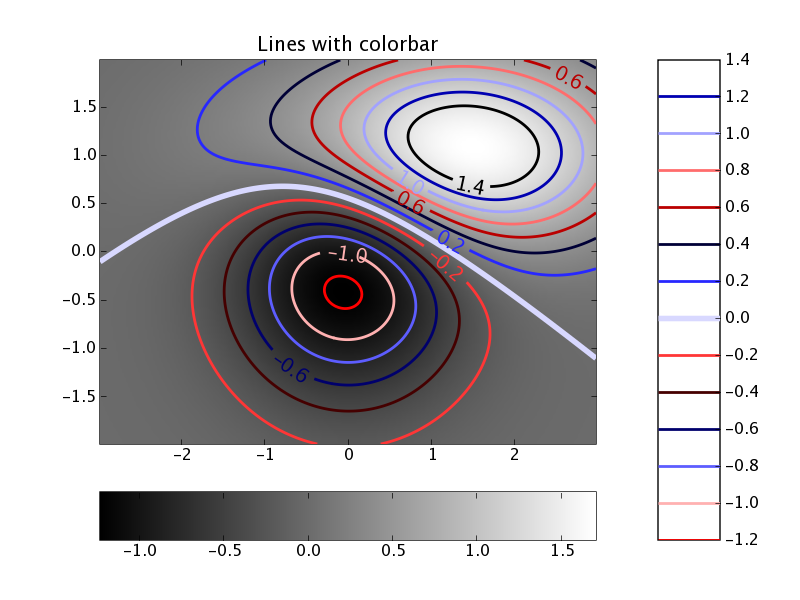
15.3.4. Plots of z = f(x, y) and other features of Matplotlib#
Matplotlib has a large number of features and can create all the standard (1d and 2d) plots such as histograms, pie charts, scatter plots, 2d-intensity plots (i.e. z = f(x, y)) and contour lines) and much more. The figure below shows such an example ([contour_demo.py] (https://matplotlib.org/stable/gallery/images_contours_and_fields/contour_demo.html)).
Some support for 3d plots is also available: https://matplotlib.org/stable/gallery/index.html#d-plotting
15.3.5. How to learn how to use Matplotlib?#
A common strategy is to scan the examples at https://matplotlib.org/stable/gallery to find a plot similar to the desired one, and then to modify the given example code. In the process, it may be worth learning more about the commands used in the example through reading the documentation.
15.4. Visual Python#
Visual Python is a Python module that makes it fairly easy to create and animate three-dimensional scenes.
Further information:
The Visual Python home page
The Visual Python documentation (explaining all objects with all their parameters)
Short videos introducing Visual Python:
Shawn Weatherford, Jeff Polak (students of Ruth Chabay): https://www.youtube.com/vpythonvideos
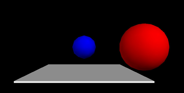
15.4.1. Basics, rotating and zooming#
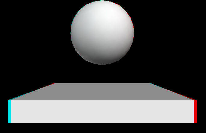
Here is an example showing how to create a red and a blue sphere at two different positions together with a flat box (vpythondemo1.py):
import visual
sphere1 = visual.sphere(pos=[0, 0, 0], color=visual.color.blue)
sphere2 = visual.sphere(pos=[5, 0, 0], color=visual.color.red, radius=2)
base = visual.box(pos=(0, -2, 0), length=8, height=0.1, width=10)
Once you have created such a visual python scene, you can
rotate the scene by pressing the right mouse button and moving the mouse
zoom in and out by pressing the middle mouse button (this could be the wheel) and moving the mouse up and down. (On some (Windows?) installations, one has to press the left and the right mouse button simultaneously and then move the move the mouse up and down to zoom.)
15.4.2. Setting the frame rate for animations#
A particular strength of Visual Python is its ability to display time-dependent data:
A very useful command is the
rate()command which ensures that a loop is only executed at a certain frame rate. Here is an example printing exactly two “Hello World”s per second (vpythondemo2.py):
import visual

for i in range(10):
    visual.rate(2)
    print("Hello World (0.5 seconds per line)")
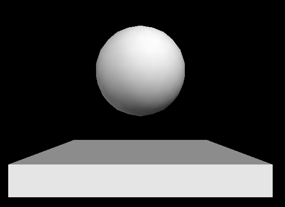
All Visual Python objects (such as the spheres and the box in the example above) have a
.posattribute which contains the position (of the centre of the object [sphere,box] or one end of the object [cylinder,helix]). Here is an example showing a sphere moving up and down (vpythondemo3.py):
import visual, math

ball = visual.sphere()
box = visual.box( pos=[0,-1,0], width=4, length=4, height=0.5 )

#tell visual not to automatically scale the image
visual.scene.autoscale = False

for i in range(1000):
    t = i*0.1
    y = math.sin(t)

    #update the ball's position
    ball.pos = [0, y, 0]

    #ensure we have only 24 frames per second
    visual.rate(24)
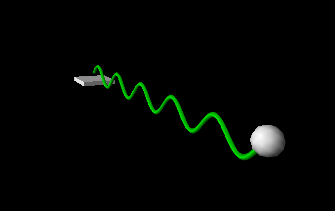
15.4.3. Tracking trajectories#
You can track the trajectory of an object using a “curve”. The basic idea is to append positions to that curve object as demonstrated in this example (vpythondemo4.py):
import visual, math

ball = visual.sphere()
box = visual.box( pos=[0,-1,0], width=4, length=4, height=0.5 )
trace=visual.curve( radius=0.2, color=visual.color.green)

for i in range(1000):
    t = i*0.1
    y = math.sin(t)

    #update the ball's position
    ball.pos = [t, y, 0]

    trace.append( ball.pos )

    #ensure we have only 24 frames per second
    visual.rate(24)
As with most visual Python objects, you can specify the colour of the curve (also per appended element!) and the radius.
15.4.4. Connecting objects (Cylinders, springs, …)#
Cylinders and helices can be used to “connect” two objects. In addition to the pos attribute (which stores the position of one end of the object), there is also an axis attribute which stores the vector pointing from pos to the other end of the object. Here is an example showing this for a cylinder: (vpythondemo5py):
import visual, math

ball1 = visual.sphere( pos = (0,0,0), radius=2 )
ball2 = visual.sphere( pos = (5,0,0), radius=2 )
connection = visual.cylinder(pos = ball1.pos, \
                             axis = ball2.pos - ball1.pos)

for t in range(100):
    #move ball2
    ball2.pos = (-t,math.sin(t),math.cos(t))

    #keep cylinder connection between ball1 and ball2
    connection.axis = ball2.pos - ball1.pos

    visual.rate(24)
15.4.5. 3d vision#
If you have access to “anaglyphic” (i.e. colored) glasses (best red-cyan but red-green or red-blue works as well), then you can switch visual python into this stereo mode by adding these two lines to the beginning of your program:
visual.scene.stereo='redcyan'
visual.scene.stereodepth=1
Note the effect of the stereodepth parameter:
stereodepth=0: 3d scene “inside” the screen (default)stereodepth=1: 3d scene at screen surface (this often looks best)stereodepth=2: 3d scene sticking out of the screen
15.5. Visualising higher dimensional data (VTK)#
Often, we need to understand data defined at 3d positions in space. The data itself is often a scalar field (such as temperature) or a 3d vector (such as velocity or magnetic field), or occasionally a tensor. For example for a 3d-vector field f defined in 3d-space (\(\vec{f}(\vec{x})\) where \(\vec{x} \in I\!\!R^3\) and \(\vec{f}(\vec{x}) \in I\!\!R^3\)) we could draw a 3d-arrow at every (grid) point in space. It is common for these data sets to be time dependent.
The probably most commonly used library in Science and Engineering to visualise such data sets is probably VTK, the Visualisation ToolKit (https://vtk.org). This is a substantial C++ library with interfaces to high level languages, including Python.
One can either call these routines directly from Python code, or write the data to disk in a format that the VTK library can read (so called vtk data files), and then use stand-alone programme such as Mayavi, ParaView and VisIt to read these data files and manipulate them (ofter with a GUI). All three of these are using the VTK library internally, and can read vtk data files.
These package is very well suited to visualise static and timedependent 2d and 3d-fields (scalar, vector and tensor fields). Two examples are shown below.
They can be used as a stand-alone executables with a GUI to visualise VTK files. It can also be scripted from a Python program, or used interactively from a Python session.
15.5.1. Mayavi, Paraview, Visit#
Mayavi Home page http://code.enthought.com/pages/mayavi-project.html
Paraview Home page https://www.paraview.org
VisIt Home page https://wci.llnl.gov/simulation/computer-codes/visit/
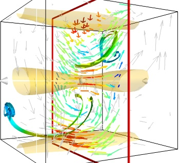
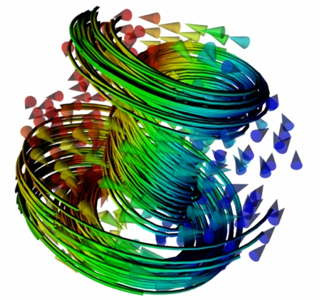
Two examples from MayaVi visualisations.
15.5.2. Writing vtk files from Python (pyvtk)#
A small but powerful Python library is pyvtk available at https://github.com/pearu/pyvtk. This allows to create vtk files from Python data structures very easily.
Given a finite element mesh or a finite difference data set in Python, one can use pyvtk to write such data into files, and then use one of the visualisation applications listed above to load the vtk files and to display and investigate them.
15.6. Further tools and developments#
In addition to matplotlib, there are a number of other libraries with similar or related visualisation functionality.
Plotly.py and Bokeh – together with the veteran of python-based plotting matplotlib – form the basis for many tools that provide visualisation skills.
A beautiful summary and categorisation of these and other libraries is available at https://pyviz.org.
15.6.1. Exploiting self-describing data for visualisation#
Some libraries, such as Pandas (see also Chapter on Pandas), Xarray, and holoviews make use of the idea of self-describing data to simplify the visualisation: while the data in a numpy array is ‘just’ a (multidimensional) matrix of data points, these libraries can store metadata – such as headings and coordinates – associated with these data points. We also talked about annotated or labelled data to describe the presence of such metadata.
What is the benefit of having this meta-data available? An xarray, for example, may store a 2d-array (like a numpy array) but have the metadata store that one dimension refers to the x-position and the other direction to time. The x-array object provides convenience methods to select and plot the data in the xarray.
15.6.2. The future of data visualisation#
I would speculate that increasingly we will be using high-level plotting tools (such as pandas, xarray, holoviews) to explore data interactively.
We can see a trend in data analysis libraries that data objects can be converted to such high-level annotated data objecs (such as European XFEL’s extra-data tools which can return a labelled xarray object). Other projects combine the metadata with the data in custom made objects to then provide convenience methods (such as Ubermag’s discretisedfield object).
Will we still need to learn the basics, such as the matplotlib.pyplot interface? Probably yes: the very least to fine tune the plots provided by these high level libraries:
15.6.3. Fine-tuning matplotlib plots that are generated by high level frame works#
We show one example where pandas – as a representative for a high-level framework that can create plots – creates the plot, but we use pyplot commands to tailor the resulting plot.
Let’s define the pandas data series first (it is not importat to understand the details of this now):
import pandas as pd
s = pd.Series(data=[10, 20, 1], index=['bananas', 'oranges', 'potatoes'])
s
bananas     10
oranges     20
potatoes     1
dtype: int64
We can use a convenience method from pandas to create a plot of the data series:
s.plot.bar()
<Axes: >

Note how the bar chart is labelled appropriately: the metadata (here the labels ‘bananas’, ‘oranges’ and ‘potatoes’) have been used to label the x-axis in the plot.
If we want to change this plot, the following strategy works, and is supported by other high-level frameworks as well:
create an axes (and figure) object
pass the axes object to the high level plotting framework
use the axes object (and figure) to finetune the plot
The following example shows how to add a title, customise the labelling of the y-axis, and add a grid to the plot, and change the size of the figure to be 10 inches by 3 inches:
import matplotlib.pyplot as plt
fig, ax = plt.subplots(figsize=(10, 3))

s.plot.bar(ax=ax, color='orange')
ax.set_title("Current stock")
ax.set_yticks(range(0, 21, 4));
ax.grid('on')

15.7. Jupyter Notebooks#
The Jupyter Notebook has become a central tool for interactive data exploration and data analysis. I would go so far to say that most data scientists will see the Jupyter notebook as the default place to start a data exploration, analysis and machine learning project.
Why is this so? The combination of annotation, code snippets, inlined results from computation or visualisation and the automatic logging of these steps in a notebook file can be of great use for research and development activities. A slightly longer summary is available here.
Some recent publications on the topic:
Brian Granger, Fernando Pérez. Jupyter: Thinking and Storytelling With Code and Data, Computing in Science & Engineering, vol. 23, no. 2, pp. 7-14, 1 March-April 2021, doi: 10.1109/MCSE.2021.3059263 Authorea preprint (2021)
Hans Fangohr, Marijan Beg, et al, Data exploration and analysis with Jupyter notebooks, Proceedings of the 17th International Conference on Accelerator and Large Experimental Physics Control Systems ICALEPCS2019, TUCPR02, doi: 10.18429/JACoW-ICALEPCS2019-TUCPR02 (pdf) (2020)
Marijan Beg; Juliette Belin; Thomas Kluyver; Alexander Konovalov; Min Ragan-Kelley; Nicolas Thiery; Hans Fangohr. Using Jupyter for Reproducible Scientific Workflows in Computing in Science & Engineering, vol. 23, no. 2, pp. 36-46, 1 March-April 2021, doi: 10.1109/MCSE.2021.3052101 arXiv preprint (2021)