Oxs Extension Module: Southampton_UniaxialAnisotropy4

The previous version of this class was called CED_UniaxialAnisotropy.

---

Description:

This is a generic Oxs extension object, derived from the Oxs_Energy class. It enhances the Oxs_UniaxialAnisotropy class as part of the standard OOMMF package by a fourth order anisotropy energy term. The energy density is computed by

E = -K₁(u·m)² - K₂(u·m)⁴,

where m is the reduced (unit) magnetization, u is the easy axis, and K1/K2 are the second/fourth order phenomenological anisotropy constants.

The corresponding anisotropy field H is given by the relation

µ₀M_sH = 2K₁(u·m)u + 4K₂(u·m)³u,

where M_s is the saturation magnetization.

For numerical reasons, the anisotropy energy density is calculated in the easy axis case (K1>0) using an equivalent form with the cross product:

E = (K₁ +2 K₂) |u×m|² - K₂|u×m|⁴.

Installation:

Download the header and source code files below, and follow the general Oxs extension installation instructions.

Usage:

MIF 2.x files written to use this class should include a Specify block of the form

Specify Southampton_UniaxialAnisotropy4:name {

K1 k1_value

K2 k2_value

axis anisotropy_axis

}

The values for the K1 and K2 parameters should be scalar field objects, and axis should be a vector field object. The only difference with respect to the stock Oxs_UniaxialAnisotropy class is the inclusion of the K2 term.

Details:

• Authors: Jürgen Zimmermann, Richard Boardman, and Hans Fangohr
• Affiliation: School of Engineering Sciences, University of Southampton
• Oxs_Ext class: Southampton_UniaxialAnisotropy4
• OOMMF releases: 1.2a3
• External libraries: none
• License: Public Domain
• Release date: 10/04/2007
• Version: 1.1 (Version 1.0 was named CED_UniaxialAnisotropy)

Download:

• C++ header file: uniaxialanisotropy4.h
• C++ main source file: uniaxialanisotropy4.cc
• Example MIF input files:
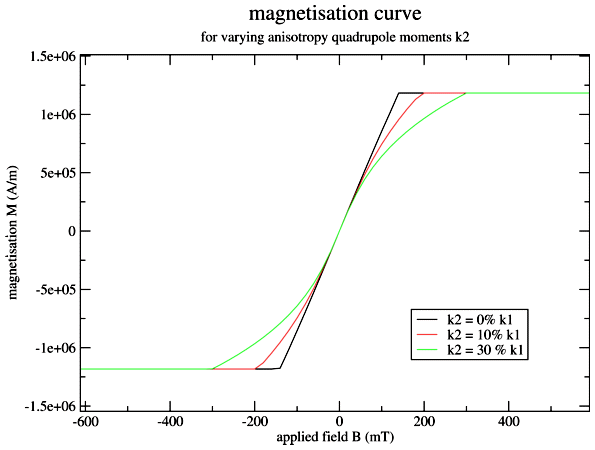
  • K2 = 0.0 K1: quadrupole00pc.mif
  • K2 = 0.1 K1: quadrupole10pc.mif
  • K2 = 0.3 K1: quadrupole30pc.mif

Sample results:

Output from the three example MIF files, illustrating the effect of increasing K2 relative to K1:

---

DISCLAIMER: This software is free to use. However, the authors do not assume responsibility whatsoever for its use, and make no guarantees, expressed or implied, about its quality, reliability, or any other characteristic.

---